| Email: info@psq.co.za Phone: 021 557 2491
|
|
|
|
Newsletter |
Demand Driven MRP and Master Production Scheduling (MPS)
by Chad Smith and Carol Ptak
What is Demand Driven MRP?
Demand Driven MRP is a new formal planning and execution method first articulated in the third edition of Orlicky’s Material Requirements Planning (Ptak and Smith, McGraw-Hill, 2011). The entire foundation of DDMRP is based upon the connection between the creation, protection and acceleration of the flow of relevant materials and information and return on investment.
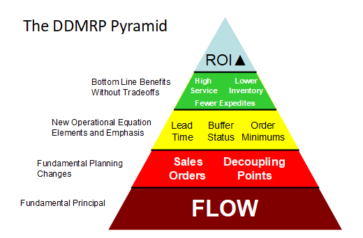
Every
for-profit company has the same goal – some form of return on
shareholder equity. When the flow of relevant materials and
information increases return on investment increases. Conversely,
when processes are drowning in oceans of irrelevant data and
materials return on investment decreases. Cash, capacity and space
is tied up in unnecessary inventory and expedite related expenses are
incurred as people attempt to deal with the chronic and frequent
shortages. Ultimately, the relevance of materials and information is
determined by whether there is a real customer demand – a demand
that results in actual payment for the effort and cash expended.
This last statement has important implications for the subject of
this article.
This article focuses on the fundamental differences between demand
inputs and capacity considerations of a DDMRP approach versus a
conventional MRP approach. The purpose of this paper is to:
- Offer an in-depth explanation of the impact of Demand Driven MRP (DDMRP) to the conventional demand input to MRP systems (Master Production Schedule).
- Explain the capacity assumptions and implications of using a DDMRP approach.
- Present the impact of DDMRP’s execution components the stability and assumptions behind an executable master schedule.
Demand Driven MRP (DDMRP) and the Master Production Schedule (MPS)
Conventional
MRP systems take their demand input from what is known as a Master
Production Schedule (MPS). The master production schedule is not
simply a statement of forecasted demand but also considers actual
sales orders, capacity and material availability. The MPS is
expressed as specific quantities and dates. Simply put, the
definition of the MPS is a statement of what
we can and will build.
MRP then takes that input and combines it with inventory records
(on-hand and open supply) and product structure (Bills of Material)
records to generate supply order requirements.
Figure 1 is a diagram from Orlicky’s Material Requirements Planning 3/E that shows how the MPS fits into the conventional MRP landscape.

As
you can see the demand input for the MPS comes from two sources;
Independent Demand Forecasts (Planned Orders) and External Orders
(Sales Orders). Traditional MRP will net the projected available
balance to zero. If the time that it takes to procure and produce
items exceeds the Customer Tolerance Time then planned orders must be
tied to supply order generation. Safety stock is used to deal with
the inherent misalignments in quantity and timing created by that
direct connection of planned orders to supply order generation. It
should be noted that the safety stock level simply becomes the "new
zero."
Master Scheduling in DDMRP
Demand
Driven MRP (DDMRP) changes the idea of a conventional MPS. In DDMRP,
the demand input is not a statement of what we can and will build but
instead it is a statement of what
we can and will sell.
DDMRP recognizes that there is a SIGNIFICANT difference in the error
rates associated with planned orders versus sales orders. Sales
orders, in most cases, are “real demand”; the equivalent of an
un-cashed check. Sales orders are the most accurate demand signals
available, representing actual demand even if the customer changes
the requirements.
Figure 2 is an equivalent diagram for the DDMRP approach. Independent Demand Forecasts are connected to the DDMRP approach ONLY through the Planned Adjustment Factors.
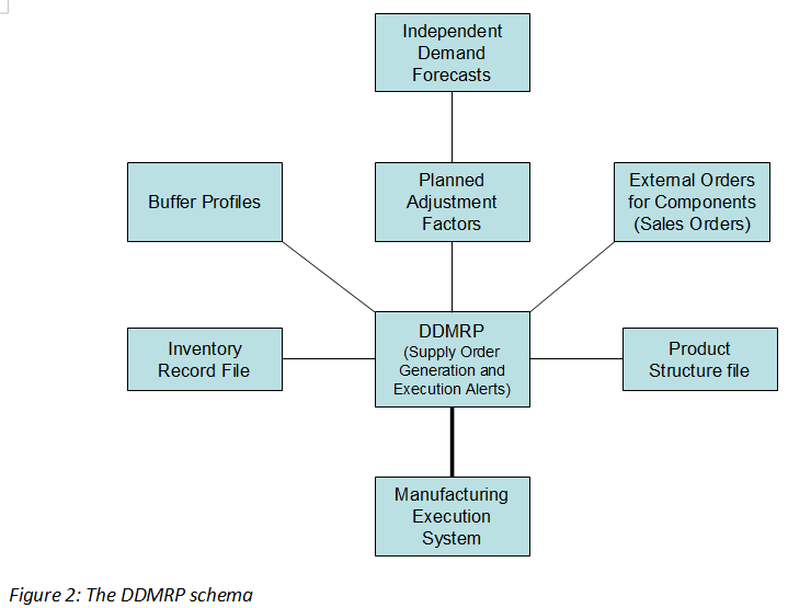
DDMRP
combines Sales Orders, Planned Adjustments, product structure
records, inventory records and buffer profiles in order to produce
recommended supply orders and execution alerts for open supply
orders. Let’s break down each component:
1.
External Orders
–actual sales order demand allocations or work order demand
allocations derived directly from actual sales orders. The DDMRP
approach further limits the consideration of external orders to
qualification criteria that will be discussed later in this paper.
2.
Planned Adjustments
– In DDMRP, actual demand orders DO NOT consume forecast. There is
no demand time fence and planning time fence to consider for forecast
consumption. In DDMRP, forecasted orders are not placed directly in
the demand equation. Forecasts are used in DDMRP but forecasts are
not tied directly to order creation. Instead DDMRP uses forecasts to
calculate Planned Adjustment Factors (PAF). The Planned Adjustment
Factors raise or lower the buffer levels, within specific time
ranges, by factoring against Average Daily Usage (ADU). ADU is a
primary component to the buffer equation. The most frequent
application of the planned adjustment factor is to dynamically adjust
buffers for a seasonal business or businesses with heavy promotional
activity.
Figure 3 depicts a planned adjustment to incorporate a temporary surge in demand either from promotional or seasonal activity. The product’s seasonal profile is displayed in monthly buckets. The left Y axis is quantity associated with the buffer levels over the course of the year. Note that the top of the buffer ranges between 700 and around 950. The right Y axis is the projected Average Daily Usage of the product over the course of the year. Below the monthly numbers is the percentage factor that will be applied to ADU within those time buckets thus creating the flex (up and down) in the buffer.
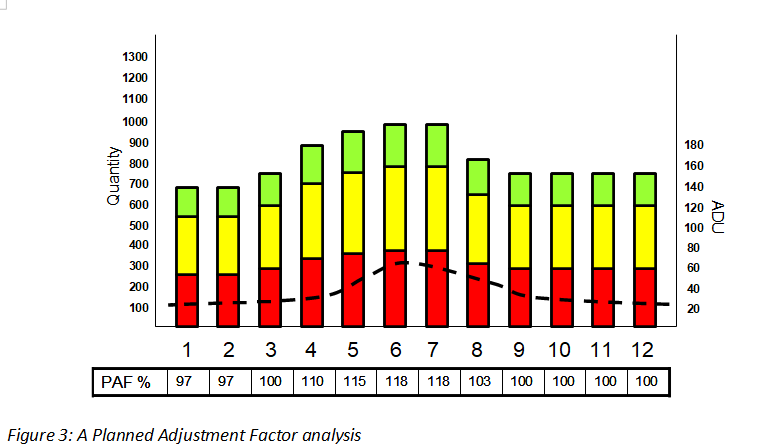
When
these planned adjustments are applied, the buffer flexes up or down
thus changing the relative available stock position of the buffer.
An available stock position of 100 for a part with no planned
adjustment factor is relatively different than an available stock
position of 100 for the same part with planned adjustment factor of
125%. When the buffer flexes up, a recommended supply order is
generated ONLY if the available stock position after the flex is
below the top of the yellow zone.
Planned
Adjustment Factors are the primary interface point between S&OP
activities and DDMRP. The application and management of Planned
Adjustment Factors is a significant topic and will be tackled in
future white papers.
3.
Buffer Profiles
– DDMRP assigns parts chosen for strategic replenishment to
families or groups based on common attributes. At a minimum, these
attributes are lead time (long, medium, short), variability (high,
medium, low), part type (made, bought, distributed) and significant
order multiple or cycle. The buffer profile the part is assigned to
affects the relative distribution of the red, yellow and green zones
of that part’s buffer.
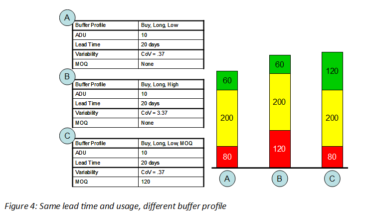
Figure 4 depicts three different parts with the same Average Daily Usage and lead time but with different profile assignments based on variability (measured through Coefficient of Variability (CoV) and minimum order quantity (MOQ).
The differences in the total buffer and the zonal distributions of the buffer depend on the part buffer profile assigned. In scenario A, the profile corresponds to a buffer profile for bought or purchased items (Buy), with a long lead time (Long) and with low variability (Low). This results in the lowest total top of buffer (called Top of Green) of 340 units (60 + 200 + 80). In scenario B the part variability is dramatically increased resulting in an increased Red Zone and a larger Top of Green. In scenario C the part has a significant Minimum Order Quantity (MOQ) which determines the size of the green zone. Not only is this buffer Top of Green larger, this buffer will have a much longer average order frequency duration (12 days on average). Average order frequency is determined by dividing the Green Zone by the ADU.
4.
Inventory Record File
– standard on-hand and open supply/on-order records.
5.
Product Structure File
– standard bill of material records.
The Net Flow Equation
These
five inputs are combined to generate recommended supply orders
through a “Net Flow equation” set against a part’s
specific buffer level and composition. The net flow equation
is unique to DDMRP.
For
end items the equation is:
(On-hand
qty) + (On-order qty) – Qualified Sales Order Demand = Net Flow Position
For
purchased and intermediate items the available stock equation is:
(On-hand qty) + (On-order qty) – Qualified Work Order Demand = Net Flow Position
Demand qualification is limited to orders that are past due, orders that are due today and orders that qualify as a demand “spike”. Spike qualification occurs by establishing an “order spike horizon” and looking for the summation of sales orders in daily buckets against a particular component/SKU that exceeds a defined “spike” threshold within the horizon. The horizon is usually set to at least one Decoupled Lead Time. Decoupled Lead Time (DLT) is defined as the summation of manufacturing lead times on the longest (measured in time) un-buffered sequence in a product’s bill of material – it is an innovation unique to DDMRP.
Figure 5 depicts the spike qualification process. In this example the order spike horizon is seven days and there are no past due orders. The order spike threshold is set at 500 units. There are orders due today totaling 400 units – those orders are qualified as demand. Additionally, there is a qualified group of orders for 1000 units that qualify as a spike that has just entered the order spike horizon. These orders are due six days after today. The entire amount of that spike is qualified as demand. In this example, today’s demand element of the available stock equation is 1,400 units.

For
intermediate components, the assumption is that the work orders
originated from a supply order from a strategic stock buffer
position. The qualification of work order demand adheres to the same
criteria as described above for sales orders.
Short Range Capacity and Materials Considerations
Any type of master scheduling (including DDMRP) makes assumptions about capacity and material availability. In the more complex and volatile environment of the 21st Century, conventional MRP’s master scheduling assumptions are becoming more unrealistic. One critical assumption of traditional MRP is that all components are available at time of order release. This is called full allocation. While conventional MPS and MRP attempt to make this occur, the combination of planned orders with certain deficiencies inherent in conventional MRP make this assumption tenuous at best. DDMRP removes these factors and assures improved flow of only relevant materials and information.
At
this point a critical difference between MRP and DDMRP is worth
noting. For strategically replenished positions, DDMRP is designed
to NEVER net the projected available balance to zero. DDMRP
specifically plans to have inventory available in order to maintain
the integrity of the buffer at the strategic decoupling point. It is
the existence of these buffers, when placed properly, that allows
lead time compression to be consistent with customer tolerance time.
These buffers also have implications for capacity consideration and
material availability.
The
existence and management of these strategic buffer positions provides
for short range capacity and materials considerations. With regard
to materials, if the buffers are designed to always have stock based
on an appropriate buffer profile then the assumption that material is
available is generally correct (especially when order spike
qualification is taken into account). For required materials or
components that are not buffered, ASR Lead Time is used to create a
realistic date for availability. The lack of the ability to
recognize ASR Lead Time is one of the critical flaws of the
conventional MRP order release calculation.
With
regard to capacity, the buffers of manufactured parts represent
stored capacity. This can act as a short range capacity buffer to
minimize capacity contention as buffers are replenished. Thus we can
make an assumption that when strategic manufactured items are
buffered, capacity is available in the short run (in the form of
stock).
Enabling Master Scheduling Assumptions with Robust Execution Elements
Now let’s turn our attention to execution. In DDMRP “planning” and “execution” are distinctly different tasks. See Figure 6 below. Planning is defined as tasks associated with generating new supply order requirements while execution is defined as tasks associated with managing open supply order requirements.

Through
an array of execution alerts, DDMRP reinforces the assumptions
contained in a reliable master schedule – that planned releases and
order synchronization will happen as planned. The existence of
these execution alerts dramatically increases visibility and focus to
potential materials, capacity and synchronization problems allowing
for preventive and/or corrective actions in order to maintain plan
and flow. Conventional MRP’s lack of integrated execution
management tools directly contributes to an often unrealistic or
unachievable master schedule.
There are 4 primary alerts used in DDMRP. Two of these alerts (Current On-Hand Alert and Projected Buffer Status Alert) are designed to be used exclusively with strategically replenished items. The Material Synchronization Alert is applicable to both strategically replenished and standard non-buffered items. The final alert is designed to be used for Lead Time Managed (strategic non-buffered) items. Figure 7 depicts the four primary execution alerts of DDMRP.

Current On-Hand Alert
The Current On-Hand Alert is designed to alert planners and buyers to current on-hand problems with strategic replenishment buffers. The alert uses color as a general reference and the percentage of a buffer’s remaining red zone as a discrete reference to generate priority status for a SKU and across SKUs. Below is an example of what a Current On-Hand Alert screen might look like. It represents the minimum amount of information necessary to display a Current On-Hand Alert.
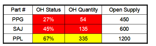
The
percentage in the status column is determined by dividing the on-hand
quantity by the top of the red zone of the buffer. In this case part
# PPG appears to be the highest priority. With only 54 units in
on-hand inventory (OH Quantity) it has only 27% of the buffer’s red
zone remaining. This means PPG’s top of red is 200 units (54/200 =
.27).
This
alert is intended to direct planner and buyer attention to the parts
with the most severely eroded buffers to highlight the supply orders
associated with them for potential expedite. In this way planners
and buyers receive a quick and easy signal of where and how to focus
their limited time.
Projected Buffer Status Alert
The Projected Buffer Status Alert is designed to warn planners and buyers about potential buffer depletions in the future based on the inventory on hand, the expected rate of use and known sales order demand over its DLT. Below is an example of what a Projected Buffer Status Alert screen might look like.

This
alert is prioritized by the short term projected future buffer status
(one DLT). It takes the quantity on-hand and compares it against
the ADU to compute a projected length of coverage until a stock out
occurs. A further level of refinement compares the total known sales
or work order demand, the release dates associated with those demand
orders and the incoming planned supply order receipts over the same
time frame to identify projected days of net negative on-hand
quantities. When a net negative position is projected using actual
demand allocations, a situation called stock-out with demand (SOWD)
is displayed. DDMRP clearly makes a distinction between SOWD and
simply being stocked out. Projected SOWD is always prioritized ahead
of projected stock outs.
In
the above example part SAJ is projected to be in a stock-out with
demand (SOWD) status in 5 days. Notice the on-hand quantity is 135
units and the ADU is 26, meaning the buffer has 5 days of coverage
remaining under average demand scenarios. Actual demand, however,
exceeds average calculated usage within the same time frame and a
supply order is not due within that period. There is total open
supply of 600 units that are candidates for potential expedite.
Something
to keep in mind about potential open supply expedites under DDMRP is
there are often multiple incoming orders against a position. DDMRP
attempts to order as frequently as possible up to the point where the
ordering becomes onerous or infeasible. Expediting smaller orders is
usually far more successful than trying to move in large orders.
Material Synchronization Alert
Material Synchronization Alerts (MSA) can involve any part (buffered or non-buffered). A Material Synchronization Alert is designed to alert buyers and planner to misalignment between any component availability and any parent release date and quantity needs. If the component quantity is expected or projected to be insufficient to meet a parent order demand allocation then an alert is triggered. Below is an example of what an MSA report, at a minimum, should provide.
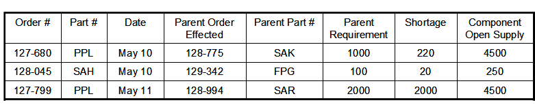
The
MSA report is sequenced by date – the more imminent the
synchronization problem, the higher the priority. PPL appears twice
on the report because it is either in short supply or its open supply
has been delayed. It is a common component to at least two
sub-assemblies (SAK and SAR). The most immediate priority is PPL’s
impact on work order #128-775. The work order requires
a total of 1000 PPLs but there will be only 780 available. The next
day work #128-994 requires 2000 PPLs and there will be none
available. There is, however, a total of 4500 units of PPL in open
supply that the buyer can choose from to attempt to expedite.
This alert allows the buyers and planners advanced warning of material/component constraints across product structures and orders. The better the visibility to these warnings the more options are at their disposal to deal with the potential conflicts. The various alerts have connections between each other. For example if PPL was a buffered item it would also appear on the Projected Buffer Status Alert as SOWD on May 10.
This alert allows the buyers and planners advanced warning of material/component constraints across product structures and orders. The better the visibility to these warnings the more options are at their disposal to deal with the potential conflicts. The various alerts have connections between each other. For example if PPL was a buffered item it would also appear on the Projected Buffer Status Alert as SOWD on May 10.
Lead Time Alert
In DDMRP the Lead Time Alert is used exclusively with strategic non-buffered parts called Lead Time Managed (LTM) parts. These are parts that are not demanded in sufficient quantity to be strategically stocked (including Engineered to Order items) but when required tend to be critical to the success of the overall project or assembly. The lead time alert is designed to provide a radar screen for planner and buyers of the impending due dates of these parts. This radar screen is a timed and structured status update to identify potential problems sooner and establish a documented order history trail.

The above graphic demonstrates the notion of a LTM part. Part PPO has been declared LTM. It has a 54 day lead time. The last third of its lead time is the lead time alert zone (18 days) and is divided into three equal portions of 6 days. Each of these portions is represented by a different color designation. Green is the farthest away from the due date. 18 days from being due the part enters the green zone of the lead time alert zone. It remains in the green zone for 6 days until day 12 when it passes to the yellow zone. Every time a LTM part enters a new color zone a Lead Time Alert is issued to the planner or buyer responsible for the part. The planner or buyer is expected to follow up on the part and input a note regarding its status. Below is an example of a Lead Time Alert report.
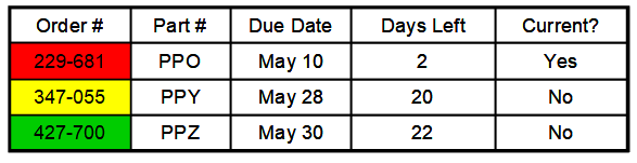
The
report will list the order numbers under a buyer or planner’s
control that are within their respective lead time alert zones.
Order # 229-681 is in the red zone. It is not late; its due date is simply
imminent. The column “Current?” is meant to distinguish parts
whose status has been updated inside the current color zone. Neither
347-055 nor 427-700 have had a status note placed against the zones
they are currently in.
The
existence of these alerts directly deals with an inherent problem
with MRP. MRP is often described as a binary system. A part is
either “OK” or “not OK”. In other words, you either have a
recommendation for action or you don’t. To make matters worse,
traditional MRP commonly gives conflicting action messages for the
same part. Moreover MRP makes no relative priority differentiation
between parts. Every day planners and buyers are drowning in action
flags and messages that are both inconsistent and/or irrelevant.
Planners know some
of the flags are important and still some matter more
than others. Getting clarity on relative priority for managing open
supply in conventional MRP is often a time consuming task and usually
involves spreadsheets, a lot of intuition and experience and even a
little luck. The execution tools inherent in DDMRP directly address
these current MRP shortfalls.
Summary
DDMRP fundamentally changes the notion of a conventional MPS. The DDMRP method provides inherently more accurate demand signals It creates an environment where the material and capacity assumptions in the plan are fundamentally more sound and the execution facilities and visibility to protect the plan against disruption.
Become a Demand Driven Planner Professional (DDPP)TM
The Demand Driven Planner Professional (DDPP)™ is a professional endorsement certification offered by the Demand Driven Institute, the global authority for Demand Driven education, training, certification and compliance. The DDPP™ is earned by an individual who can apply the demand driven concepts, analyze an environment and evaluate an environment using the Demand Driven Material Requirements Planning (DDMRP) methodology. See https://www.demanddriveninstitute.com/demand-driven-planner-ddp. The next 2 day DDP course in Cape Town is scheduled for 6-7 November 2018.
Content copyright © Demand Driven Institute - used with permission.