The Power of Decoupling

Unlocking the Secret to Demand Driven Material Requirements Planning (DDMRP)

By Chad Smith

Building a Foundation of Flow

The recognition of manufacturing as a process is essential to understanding how it should work. Understanding how it should work gives us the capability, in light of current conditions, to define what the rules surrounding it should be. Which rules need to stay? Which need to go? Which need to change? Which need to be added?

Manufacturing is a bewildering and distracting variety of products, materials, technology, machines, and people skills obscuring the underlying elegance and simplicity of it as a process. The essence of manufacturing (and supply chain in general) is the flow of materials from suppliers, through plants, through distribution channels to customers, and of information to all parties about what is planned and required, what is happening, what has happened, and what should happen next.

An appreciation of this elegance and simplicity brings us to what George Plossl (a founding father of MRP and author of the second edition of Orlicky’s Material Requirements Planning) articulated as the First Law of Manufacturing: All benefits will be directly related to the speed of flow of information and materials.

“All benefits” is quite an encompassing statement. What does “all benefits” really mean? Let’s break it down into components that most companies measure and emphasize. All benefits encompasses:

Service. A system that flows well produces consistent and reliable results. This has implications for meeting customer expectations not only on delivery performance but also on quality. This is especially true for industries that have shelf-life issues. Do you want to dine at the restaurant that has poor flow or great flow?
Revenue. When service is consistently high, market share grows or, at a minimum, doesn’t erode.
Inventories. Raw and pack, work-in-process, and finished goods inventories will be minimized and directly proportional to the amount of time it takes to flow between stages and through the total system. The less time it takes products to flow through the system, the less the total inventory investment (exploring Little’s Law will help in understanding this point).
Expenses. When flow is poor, additional activities and expenses are incurred to close the gaps in flow. Examples would be expedited freight, overtime, rework, cross-shipping, and unplanned partial ships. Most of these activities directly cause cash to leave the organization and are indicative of an inefficient overall system. In many companies, these expedite-related expenses are underappreciated and under-measured.
Cash. When flow is maximized, material that a company paid for is converted to cash at a relatively quick and consistent rate. This makes cash flow much easier to manage and predict. Additionally, the expedite-related expenses previously mentioned are minimized.

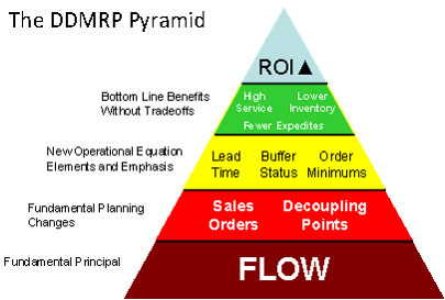
What happens when revenue is growing, inventory is minimized and additional and/or unnecessary ancillary expenses are eliminated? Return on Investment (ROI) moves in a favorable direction! And isn’t that really the objective? Every for profit company has a universal primary goal; to protect and promote some form of return on shareholder equity. What’s the best, sustainable way to do that? PROMOTE AND PROTECT FLOW. This is the very definition of a truly effective manufacturing system.

But there is an important caveat to the first law that becomes crucial and central to make these things happen. The flow of information and materials must be RELEVANT to the output or market expectation of the system. The great basketball coach John Wooden said, “Never mistake activity for achievement.” We can’t just indiscriminately move “information” and materials quickly around a system and expect it to be effective. What we frequently observe is organizations drowning in oceans of data with little relevant information and large stocks of irrelevant materials (too much of the wrong stuff) and not enough relevant materials (too little of the right stuff). When this occurs there is a direct and adverse effect to return on investment.

Is the concept of promoting the flow of relevant information and materials difficult for people to grasp? Titans of early industry like Henry Ford, F. Donaldson Brown and Frederick Taylor all understood this importance and built their models around it; models that provided the backbone of modern corporate structure. Later thought leaders such as Plossl, Ohno, Deming and Goldratt built entire methodologies around the concept. The concept is a basic tenet of management accounting. The concept is also intuitive. In general most people within an organization seem to intuitively grasp why flow is so important. It’s simply too difficult to foster flow using conventional MRP systems in the set of circumstances that we are faced with today.

Conventional Planning Systems and the Bi-Modal Reality

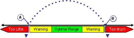
Do conventional planning systems protect and promote the flow of RELEVANT information and materials? Our research suggests that they do not. Experienced planning and purchasing personnel see the evidence every day in front of them. In order to illustrate what they see we will use a simple graphical depiction. Below you see a line running in both directions. This line represents quantity of inventory. As you move from left to right the quantity of inventory increases; right to left the quantity decreases.

Whether it is at the single SKU/Part # level or at the aggregate inventory level, there are two very important points on this curve:

A point where we have too much inventory and there is excess cash, capacity and space is tied up in working capital. This is represented by point B.
A point where we have too little inventory and the company experiences shortages, expedites and missed sales. This is represented by point A.

If we know that these two points exist then we can also conclude that for each SKU/Part #, as well as the aggregate inventory level, there is an optimal zone somewhere between those two points. This optimal zone is depicted below in green. Most planners and buyers want to operate right there – a place where they are safe from stock-outs and expedites AND don’t get called to the carpet for excessive amounts of inventory. But can they?

As the inventory quantity expands out of the optimal zone and moves towards point B the return on the working capital captured in the inventory becomes less and less. The converse is also true as inventory shrinks out of the optimal zone and approaches zero or less than zero and our service risk grows. Placing point A at the quantity of zero means that inventory becomes too little when we are stocked out. Placing Point A at less than zero means that inventory becomes too little when we are “stocked out with demand” – the traditional definition of a true shortage.

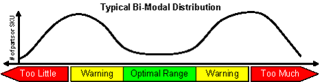
When the aggregate inventory position is considered against these zones we frequently notice a bi-modal distribution in which a large number of SKU/part #s have too little while still another large number have too much inventory. The smallest population tends to be in the optimal zone.

Not only is the smallest population in the optimal zone, the time any individual SKU spends in the optimal zone tends to be short lived. In fact, most SKUs tend to oscillate between the two extremes. That oscillation can occur in an extremely short time frame, especially when planning using traditional forecasted demand, safety stocks and weekly MRP runs.

This oscillation distorts, obscures and hides the flow of relevant information and materials. Planners and buyers are drowning in action flags and reschedule messages. They know that if they acted on everything they would simply reverse many of those actions in the near term future or worse, create even more detrimental and unforeseeable effects. They know some things are very important while others simply don’t matter but they cannot determine what is relevant and truly important.

The bimodal distribution results in three simultaneous effects that negatively impact return on investment:

Unacceptable inventory performance – too much of the wrong inventory creating low turns and obsolescence risks.

Chronic and frequent shortages – missed sales and schedule slides due to too little of the right inventory.

Accommodating expenses – all of the expenses we incur in reaction to the bimodal effect:

Expedited freight from suppliers
Overtime on the shop floor to make up for schedule slides
Additional freight because we shipped partials
Additional warehousing space

All of these effects directly relate to or impede the benefits that we described inherent to the protection and promotion of flow. When that happens ROI is compromised.

Is this bi-modal distribution real? The results of our surveys is quite compelling. With over 500 different companies responding, nearly 90% report that the bimodal effect is occurring in their operations. What will it take to break down this bimodal distribution and promote and protect the flow of relevant information and materials?

System Variability – Enemy #1 to Flow

If sustainable financial return is related directly to our ability to protect and promote the flow of relevant information and materials then we need to understand what the biggest enemy to that flow is.

The answer simply stated is system variability. The impact of variability must be better understood at the systemic rather than the discrete process level. The war on variability that has waged for decades has most often been focused at a discrete process level with little focus or impact to the total system. Variability at a local level in and of itself does not impede system flow. What impedes system flow is the accumulation and amplification of variability. Accumulation and amplification happens due to the nature of the system, the manner in which the discrete areas interact (or fail to interact) with each other. The Law of System Variability states that

The more that variability is passed between discrete areas, steps or processes in a system, the less productive that system will be; the more areas, steps or processes and connections between them the more erosive the effect to system productivity.

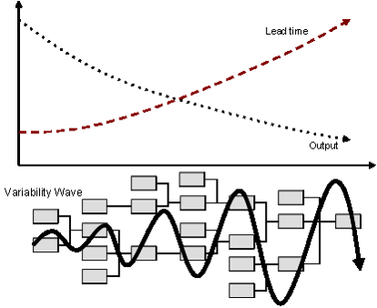
The figure above illustrates the Law of System Variability. The lower half of the graphic depicts a network of connections. It could represent a project network, a supply chain, a bill of material or even a routing. It depicts a set of relationships between discrete events, areas or entities that culminates in some form of completed product, project or end state. The large squiggly crescendo line represents a variability wave that accumulates and amplifies through the system; delays are frequently accumulated while gains are rarely accumulated. The graph above the network section shows the impact of the variability wave to system lead time and output. In short; lead time expands while output decays. Significant resources are expended trying to pull the ends of those arrows together.

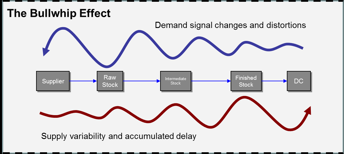
At the supply chain level this lesson manifests itself as something called the bullwhip effect. The bullwhip is a rather infamous effect in industries with large extended supply chains dominated by major assemblers. Examples would include aerospace, automotive and consumer electronics. Distortions and changes in demand signals move from right to left (customer to supplier) while delays and shortages are passed from left to right (supplier to customer). The figure below illustrates the Bullwhip Effect.

Decoupling – the Key to Demand Driven Material Requirements Planning (DDMRP)

If the accumulation and amplification of variability is the biggest enemy to system flow then we have to design a system that that stops or mitigates the transfer and amplification of variability through the system. But how to do that? The answer cannot be “guess better” or “eliminate all variability.” Industry has tried that for decades, has spent fortunes and failed.

The concept of “decoupling” provides the break from convention that is needed. Decoupling breaks the direct connection between dependencies. The places at which we decouple are called “decoupling point.”

Decoupling point—the location in the product structure or distribution network where strategic inventory is placed to create independence between processes or entities. Selection of decoupling points is a strategic decision that determines customer lead times and inventory investment.

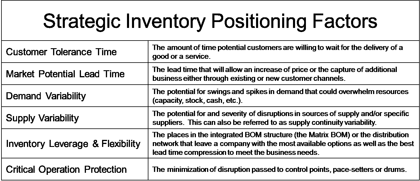
Decoupling points represent a place to disconnect the events happening on one side from the events happening on the other side. They delineate the boundaries of at least two independently planned and managed horizons. Where to place these decoupling points? The answer is neither “everywhere” nor “nowhere.” The answer is simply stated as “somewhere.” But how to find that somewhere? Where to strategically place decoupling points depends on careful consideration of the six factors in Table 1.

Table 1: Decoupling Point Selection Criteria

Unfortunately conventional planning systems are not set up to position and then manage decoupling points. The very basic foundation of Material Requirements Planning (MRP) was to make everything dependent – decoupling is a not a word in its vernacular. When we look deeper we see that the inability to decouple is the primary culprit behind system variability in planning systems and a major impediment to flow.

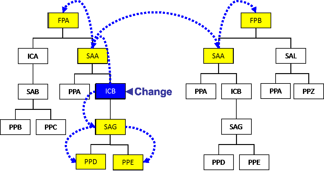
MRP’s nature of making everything dependent creates something called “nervousness.” Nervousness is the characteristic in an MRP system related to changes at any level transferring up, down and across bills of material. The figure below illustrates nervousness. When change is introduced at Intermediate Component B (ICB) it has a ripple effect up and down Finished Product A’s (FPA) bill of material and also across to impact Finished Product B (FPB). This will typically result in both quantity and timing changes for both product structures. This is the very cause of the oscillation effect that occurs in the bimodal distribution.

Mitigating variability and thus promoting and protecting the flow of relevant information and materials requires decoupling. There is simply no alternative if we want to drive to a goal of maximizing shareholder equity and return on working capital.

Decoupling simply makes sense given the basic circumstances that we face today. We have elongated and more complex supply chains. These longer and more complex supply chains are subject to much higher levels of variability and much harder to plan. Breaking dependencies in key places will dramatically simplify the planning equation and allow us to live in shorter horizons with much more relevant information.

One of the most obvious things that has occurred in supply chain over the last two decades is that customer tolerance times are becoming shorter in relation to our elongated and complex supply chains. With this in mind we reach a simple conclusion; someone has to hold stock somewhere. Not everywhere. Not nowhere. Somewhere. The natural place to put this stock is at the decoupling points.

Decoupling Point Buffers

In order to make decoupling points absorb variation from both supply and demand direction (thus making them truly independent) a cushion or dampening mechanism must be used. This dampening mechanism is called a “buffer”. This buffer takes the form of stock and serves to compress lead time and dampen variability.

By decoupling supplying lead times from the consumption side of the buffer, lead times are instantly compressed. This lead time compression has immediate service and inventory implications. Market opportunities can be exploited while working capital required in buffers placed at higher levels in the product structure can minimized.

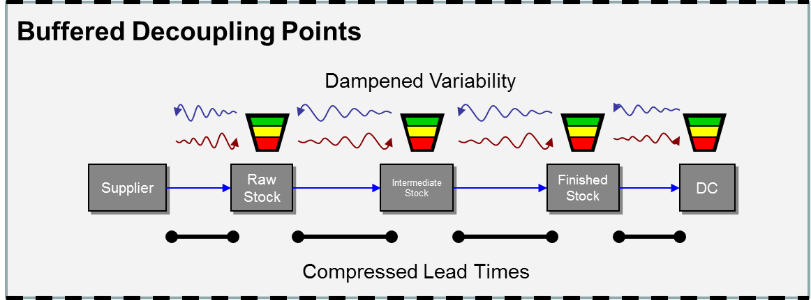
As seen in the figure above stock buffers are designed to provide bi-directional dampening of variability to significantly reduce or eliminate the bullwhip effect. By planning for stock to be maintained at decoupling points the consumption of this stock can remain independent from the supply for a certain period of time. It is important to note that the stock contained in these positions are “order independent” – meaning the stock is at the discrete part number level. It is not WIP and is available on demand to all potential parent item or sales order demand that may call for it.

Stock buffers initially are sized through a combination of factors including an average rate of use, lead time, variability, and order multiples. Then the buffers are stratified into color zones (green, yellow, and red) for easy priority determination in planning and execution. Each zone has a specific purpose and will vary in size and proportion depending on the “buffer profile” that the buffered part has been assigned. The buffer profile is a group of settings applied to a group of parts that have similar attributes. In practice we expect to see globally managed groups of parts with different combinations of these attributes:

Part Type (made, bought or distributed)
Lead time (long, medium, short)
Variability (high, medium, low)
Large Order Multiples (relative to usage)

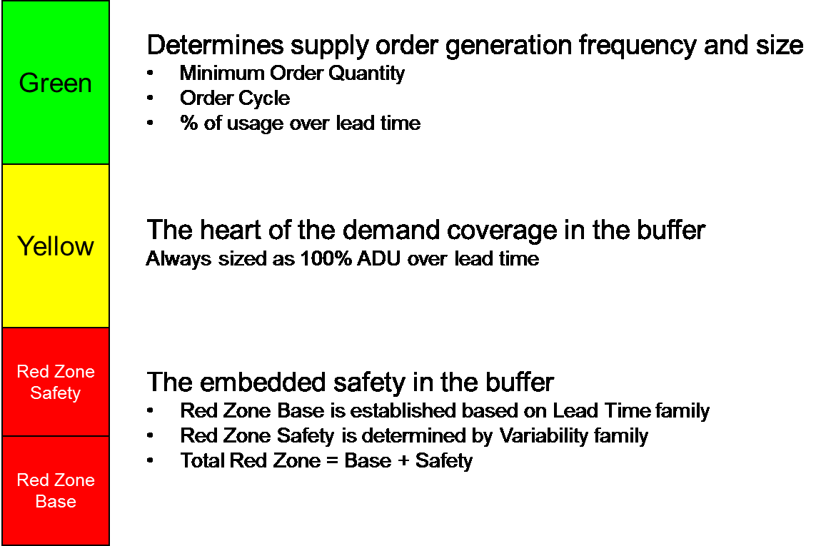
As mentioned above, each zone in the buffer has a purpose and is sized by various elements of the profile. Below is a quick reference chart that describes the purpose of each zone and the elements that go into the sizing. These buffers dynamically adjust with market changes in consumption or in advance of planned or known activity, such as seasonality or large promotional activity.

A critical element to point out in the figure above is the role of the buffer’s green zone – to determine supply order generation frequency and size. Through the green zones the buffers actually become the primary planning mechanism.

A New Way for Supply Order Generation

In addition to lead time compression and variability dampening, the buffers placed at the decoupling points are the heart of supply order generation for Demand Driven MRP. They become a focal point for creating, promoting, protecting and determining relevant information and materials. They also create the opportunity for a much more elegant and visible way to generate supply orders.

Decoupling Supply Order Generation From Forecast – Supply chain and manufacturing planning always starts with a demand signal. Unfortunately when you start a serial, complex and interdependent process with an infrequent and error prone input, the result of the process will be unsatisfactory. The waste and performance erosion associated with that inaccuracy will simply grow in magnitude. In order to provide the best possible input to the supply order generation process we will need to address both the nature of the signal as well as the frequency of the signal.

Based on a given demand signal, MRP is designed to net perfectly to zero. You make exactly what you need without any excess. It could be argued that MRP is the perfect JIT system. If the demand signal is perfectly accurate then the MRP calculation will be perfectly accurate. Given the math allows no room for error, it seems obvious that MRP should only be given as accurate a signal as possible.

The most accurate form of demand input is a sales order. A sales order is a stated intention and commitment by an actual customer of need in terms of quantity and time. It defines what is relevant both in terms of information and materials. There is no debate that sales orders are an order of magnitude more accurate than planned orders. So why don’t companies simply load only sales orders into MRP?

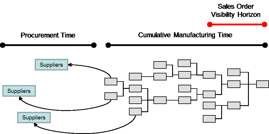
Using MRP with only sales orders, however, assumes something that does not exist in today’s environment – enough time. In order for MRP to be that perfect JIT system, you must have the time to procure and make everything – called cumulative lead time (the longest stated chain of time in the bill of material including purchasing lead time). Customer tolerance time would have to be equal to or greater than cumulative lead time. Today’s supply chains, however, are characterized by shorter and shorter customer tolerance times and extended, elongated and increasingly complex supply chains. We simply don’t get visibility to sales orders soon enough to properly plan for them using conventional MRP. How must we make up for the widening gap between the time it takes to procure and produce and the lead time that customers demand?

With MRP’s characteristic of making everything dependent the only way to find enough time is to attempt to predict what actual demand will look like so that we can attempt to ensure the necessary materials in quantity and time as the market places its sales orders. Thus, the need to load MRP with demand that is largely derived from forecast.

There are three truths about forecasts:

All forecasts start out with some inherent level of inaccuracy
The more remote in time or farther out forecasts go, the less accurate they get
The more detailed or discrete the forecast is the less accurate it will be

Planned Orders are commitments of cash, capacity and/or materials directly derived from a prediction that is subject to varying degrees of inaccuracy. As time progresses, the demand picture changes, MRP is rerun and nervousness occurs. The result is we end up with things we do not need and desperately expedite things we have just discovered that we do need. The bimodal distribution starts with the use of planned orders!

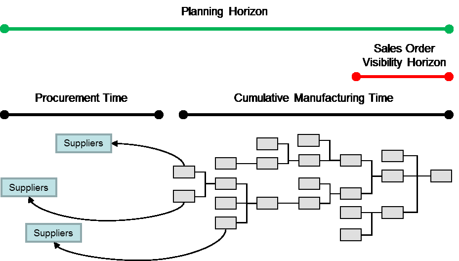
The assumption that that the only way to find the time is to use planned orders derived from forecast is only true due to MRP’s basic nature to make everything dependent. Yet, when we consider the power of decoupling we find the way to be able to use actual orders (sales orders). Remember, decoupling creates independence between supply and demand and where we decouple directly effects our lead time to market. The closer we can place a decoupling point to when sales orders become visible, the more accurate the demand signal AND the better the response to the market.

As previously mentioned, the buffers placed at decoupling points represent a cushion that allows us to block or stop the accumulation and amplification of variability – they buy us the time we so desperately need to meet actual customer expectations and to use sales orders as the basis for our demand signal input. Now we have to understand how to maintain those buffers in a way that does not penalize us with excess inventory yet creates timely and accurate demand signals (relevant information) for their replenishment (relevant materials).

Decoupling From the Weekly Bucket – In most environments planning occurs in weekly buckets. This is a direct effect of the nervousness discussed above – nervousness that is directly related to the inability to decouple. Planning organizations know that if they ran MRP daily the resulting nervousness would create chaos. The amount of action flags and messages on the planning screens would be overwhelming.

Instead a weekly interval is used to calm the waters on a daily level. This, however, comes at a price. First, it forces the planning horizon to extend. This has a direct correlation to the level of signal inaccuracy at the end of the horizon. Second, it creates a latency that almost guarantees that the level of change between MRP runs will be dramatically larger. Instead of lots of little changes on a daily basis, we get massive changes on a weekly basis. Planning organizations are stuck between these two hard places because MRP’s hard coded trait of making everything dependent.

Decoupling opens a door to end this compromise where daily planning becomes obvious, intuitive and beneficial for supply order generation.

Demand Driven MRP Supply Order Generation – In order to produce relevant information for relevant materials, the DDMRP planning process shifts to daily planning buckets. This does not mean that all buffered parts will be ordered every day. It does mean that in most environments some supply orders will be generated every day against some of the buffered items. What will dictate how many supply orders are generated every day is a review of the net flow position of each buffered item. That position is reviewed on all buffered parts every day.

The net flow position is determined by a unique supply order generation equation called the net flow equation. All qualified demand, supply and on-hand information are combined at the buffer to produce the net flow position for buffered items. The net flow equation is relatively simple to understand but foreign to conventional planning systems.

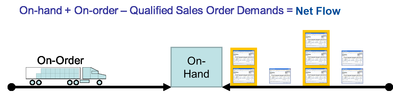
The net flow equation adds open supply to on-hand and then subtracts qualified sales-order demand. The figure above graphically demonstrates the net flow equation. In the middle is on-hand – physically available inventory. On the left is on-order – the quantity of stock that has been ordered but not received regardless of due date. On the right is qualified sales order demand. Qualified sales order demand is limited to sales orders due today, due in the past, and future qualified spikes. The highlighted sales orders in yellow are qualified demand. Two are due today and three that are due two days from now (on day three) represent a qualified spike. To qualify a spike two conditions must be met. The amount of sales order demand must be above the order spike threshold and the sales order must be due within the order spike horizon.

The order spike threshold is a level that qualifies a spike in a particular environment. The summation of sales orders (for the same part number) for each day is totaled and compared against the threshold. If the summation is greater than the threshold than the entire amount (not just the amount above the threshold) is incorporated into the net flow equation as a qualified spike. An order spike threshold is depicted in the figure below by the horizontal dotted line. Two days from today (marked day 3) the three sales orders due on that day represent enough combined demand to qualify as a spike.

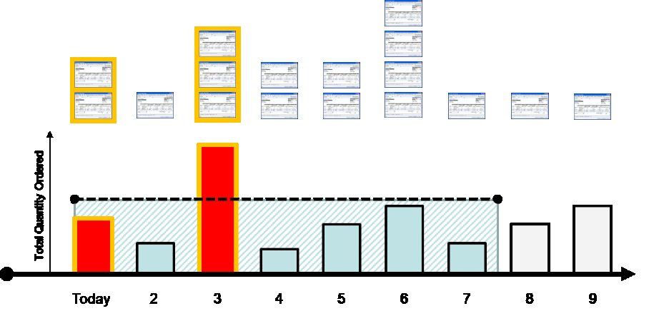
The second condition is also met by these three sales orders on day 3. They are within the order spike horizon. In the figure above, the order spike horizon is set to seven days. It is represented by the length of the dotted line.

There are several sales orders in several daily buckets that are within the order spike horizon but do not qualify as a spike. The four orders on day six, for example, do not total to greater than the threshold.

Now the obvious question – why not include all known sales orders in the net flow equation? The answer is simple. They are essentially already accounted for in the buffer! If the daily sales order demand is under threshold, they represent relatively normal or average demand. How did we build the buffer levels? We built them using equations with average rate of use. Thus, what is due today, due in the past and what is qualified as a spike is really all that is relevant from a demand perspective.

Supply orders are only created when the net flow equation produces an net flow position below the top of the yellow zone. Supply orders are then recommended in a quantity to restore the net flow to the top of the green zone. The figure below is an example of a daily planning DDMRP planning screen.

Part	Open Supply	On-hand	Demand	net flow	Recommended Supply Qty	Action
f576	3358	4054	540	6872	3128	Place New Order
h654	530	3721	213	4038	2162	Place New Order
r457	5453	4012	1200	8265	0	No Action

There are three parts depicted on this screen. The screen displays the relevant components of the net flow equation and then displays the net flow position and the zonal color of the buffer that position falls in. For example, part r457 has open supply of 5453, on-hand of 4012 and qualified demand of 1200. This yields an net flow position of 8265 (5453 + 4012 – 1200).

Only two of the parts are relevant from a supply order generation perspective (f576 and h654). Both have an net flow position within the yellow zone (under top of the yellow). Supply orders are recommended for each of these parts to restore their net flow positions to the top of their respective green zones. If these orders are accepted their net flow statuses will go to green.

Part	Open Supply	On-hand	Demand	net flow	Recommended Supply Qty	Action
r457	5453	2812	2100	6165	4512	Place New Order
f576	6486	3514	710	9290	0	No Action
h654	2692	3508	305	5895	0	No Action

Tomorrow when we review the planning screen (depicted by the figure above) we find new net flow positions for each of our three parts. On hand amounts have been adjusted for all parts by the amount of demand fulfilled in the previous day (in our example all qualified demand yesterday was due yesterday – there were no qualified spikes). New demand amounts have been qualified. Open supply for f576 and h654 have increased by yesterday’s approved supply orders respectively. The net flow status for r457 has now gone yellow and a supply order in the amount of 4512 is recommended.

Decoupled Explosion – When considering decoupling and the DDMRP supply order generation process an obvious impact emerges. When a supply order is generated at a higher level decoupling stops the explosion of a bill of material at decoupling points placed at lower levels. The explosion can be stopped because the decoupling point is buffered. Consumption and demand can be accumulated at that point until resupply is recommended through the net flow equation. The explosion then begins again relative to that part’s respective components.

This concept is crucial in preventing nervousness because most changes at high level parents will not be big enough to pass through the buffers and thus create the nervousness that destroys flow. This is especially true for decoupling points placed at common components (a common strategy) as we get the smoothing benefit of aggregation.

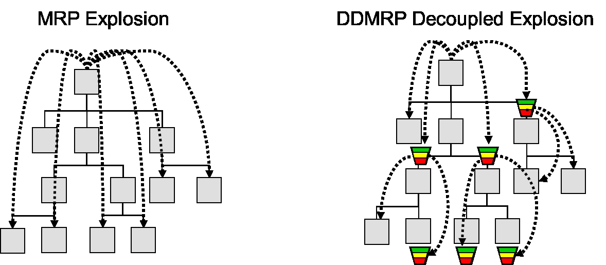
This creates an effect called a decoupled explosion depicted by the figure on the right in the graphic above. Decoupled explosion is a critical distinguishing characteristic of a DDMRP system. It is important to understand that there is a combination of dependence and independence. There is independence at the decoupling points but between decoupling points there is dependence that is no different than conventional MRP.

The figure on the left represents conventional MRP where any change at the higher level is typically driven all the way through to the purchased level. There are some exceptions to this rule in MRP but they are simply that – exceptions. Decoupled explosion is a cornerstone of planning mechanism in a DDMRP system and allows the flow of relevant information and materials to be promoted and protected.

A Final Note on DDMRP Buffers

Commonly DDMRP stock buffers are confused with mechanisms like safety stock, kanbans and order point. These comparisons are understandable but inaccurate.

DDMRP buffers versus safety stock – Safety stock does not decouple--it seeks only to compensate for variability, assuming no decoupling or lead-time compression (i.e., a longer planning horizon). This makes it an inefficient type of dampening mechanism. Additionally, safety stock often has mechanisms (such as order launches and expedites) that can exacerbate the bullwhip effect.

DDMRP buffers versus order point – Order point systems typically do not take into account actual demand. Order point determines resupply through the incorporation of on-hand and open supply only. By failing to include qualified demand in the equation, order point positions are more vulnerable to demand spikes. Additionally, order point incorporates a safety stock mechanism that often results in additional and often unnecessary expedited supply orders.

DDMRP buffers versus kanban – Technically kanbans are work in process positions and are placed in front of resources. This can force inventory to spread everywhere and dramatically complicate the ability to resize the positions based on changes in the environment. Kanbans can be slow or inadequate to respond to spikes or seasonality.

It is worth noting that the typical implementation of stock buffers at strategically determined control points does NOT typically raise inventory in a system. Early adopters across many diverse industry segments adopting the DDMRP methodology have realized 20-60% reductions in total inventory while simultaneously increasing service levels. This has served to reinforce the power and direct connection to ROI of flow within early adopters of this methodology.

Summary

Today’s companies are held hostage by hard-coded rules in MRP - rules that act as a foundation for the way MRP functions - rules that have been around since the inception of MRP in the 1950’s. Many of which directly result in the distortion and obfuscation of relevant information for planning personnel and lead directly into materials challenges evident in the bimodal distribution. This impediment to the flow of relevant information and materials directly compromises the protection and promotion of sustainable return on investment.

Perhaps one of the most damaging rules is MRP’s inability to decouple. The concept of decoupling and decoupling points is not new. Both terms have been correctly defined in the APICS dictionary for decades. However, the practical and standardized application of decoupling under DDMRP is new.

Rooted in a foundation of flow, the concept of decoupling unlocks the door for much more effective planning. It gives us the capability to use the highly accurate demand signals we have had available to us for years – sales orders. When used properly, decoupling effectively ends nervousness by stopping variation from being passed within the supply chain. When the supply chain has significantly less nervousness, things become clearer and determining what is relevant becomes an order of magnitude easier. Thus decoupling becomes the first step to driving the promotion and protection of the flow of relevant materials and information that is so crucial for driving improved return on investment performance.

About the Author

Chad Smith is the co-author of the third edition of Orlicky’s Material Requirements Planning 3/E (Ptak and Smith, McGraw-Hill, 2011), Demand Driven Performance – Using Smart Metrics (Smith and Smith, McGraw-Hill, 2013) and Demand Driven Material Requirements Planning (Ptak and Smith, Industrial Press, 2016). He is a co-founder and Partner in the Demand Driven Institute, an organization dedicated to proliferating demand driven methods throughout the world. Chad served as the Program Director of the International Supply Chain Education Alliance’s Certified Demand Driven Planner (CDDP) Program from 2012 to 2016.

References
Blackstone. (2013). APICS Dictionary (Fourteenth Edition). Chicago: APICS.
Plossl, G. (1994). Orlicky's Material Requirements Planning. McGraw-Hill.
Smith, C., & Ptak, C. (2011). Orlicky's Material Requirements Planning. McGraw-Hill.
Smith, D., & Smith, C. (2013). Demand Driven Performance - Using Smart Metrics. McGraw-Hill.

Content copyright � Demand Driven Institute - used with permission.

For further information, contact Colin Seftel